Producing Automated Outputs (using R)

Presenter(s): Leo Westbury

Types of statistical results tables

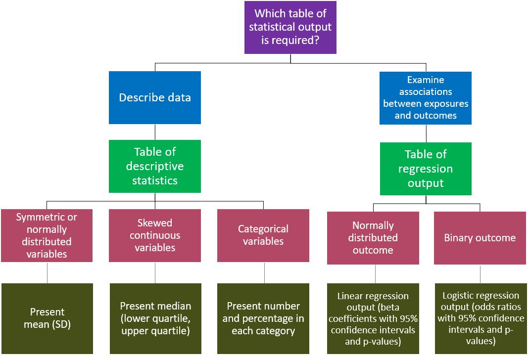
The type of results table to produce will depend on whether the analysis is descriptive or aims to examine associations between exposures and outcomes, and also on whether the variables of interest are continuous or categorical. The flowchart, below, suggests the appropriate type of table to produce, depending on these factors.

> Download this flowchart as a PowerPoint file, for accessibility.

Installation of R

R can be downloaded and installed from The Comprehensive R Archive Network (r-project.org) for Windows, macOS and Linux users. Once you have selected your operating system, you can click on the link install R for the first time; this will download the R executable (.exe) file. You can then run this file and follow the instructions to install R. You may be prompted to select a CRAN mirror location to specify the location of the server to use for downloading R software or packages. It is good practice to select a CRAN mirror which is close to your current location as this will improve the download speed.

 

Creating a script file in R

A script file is a text file which enables users to document a sequence of R commands to be run. For example, a script file may load some R libraries that contain certain functions, then import a dataset and then output descriptive statistics for variables in this dataset. Script files allow users to efficiently record their R code and ensure that their analyses are reproducible.

To create a script file, click File and then click New script. To run the script file, click on this icon:

Installation of packages and initial data preparation

The first step is to install the required packages and load them using the library command. The packages only need to be installed once but they will need to be loaded at the start of every R session. Therefore, the code below should be run at the top of your R script before running any of the commands in this online resource. However, as the install.packages function only needs to be run once, it can be deleted from your script after the packages have been installed. If you do not have permission to install packages to a system-wide library (for all users of the computer), you may be prompted to create a personal library to install the packages into.

#Install and load required packages
install.packages("gtsummary")
install.packages("flextable")
install.packages("officer")
install.packages("car")
library(gtsummary)
library(flextable)
library(officer)
library(car)

> Download the complete code in this resource, as a single Word Document file.

 

The mtcars dataset (part of the car package) can then be loaded and manipulated prior to producing any tables. After loading this dataset, some variables that we are not interested in are removed; the variables retained for analysis are presented in the table directly below. The code below loads the dataset and performs the necessary manipulations prior to producing the tables.

Variables retained for analysis in the mtcars dataset

Variable	Definition
mpg	Fuel economy (miles per gallon)
cyl	Number of cylinders
wt	Weight in tonnes
vs	Engine configuration (0: V-shaped   1: Straight)
am	Transmission (0: Automatic   1: Manual)

 

#Create a dataset called 'cars' by loading the built-in 'mtcars' dataset
#Some variables are then removed to create a smaller dataset
cars <- mtcars
head(cars)
cars$drat<-NULL
cars$qsec<-NULL
cars$hp<-NULL
cars$gear<-NULL
cars$carb<-NULL
cars$disp<-NULL
head(cars)
summary(cars)

#Examine distribution of variables
hist(cars$mpg)  # Approximately normally distributed 
table(cars$cyl) # Values of 4, 6, 8 
hist(cars$wt)   # Continuous, not normally distributed 
table(cars$vs)  # Values of 0, 1 
table(cars$am)  # Values of 0, 1       

#Convert weight from 1000s of pounds to tonnes
cars$wt <- cars$wt * 0.454

#Declare categorical variables as factor variables and label the categories
cars$vs     <- factor(cars$vs, levels = c(0,1), labels = c("V-shaped", "Straight"))
cars$am     <- factor(cars$am, levels = c(0,1), labels = c("Automatic", "Manual"))
cars$cyl    <- factor(cars$cyl, levels = c(4,6,8))

#Re-order dataset columns and examine final dataset
cars <- cars[, c("am", "wt", "vs", "cyl", "mpg")]
head(cars)
summary(cars)

 

Produce tables of descriptive statistics

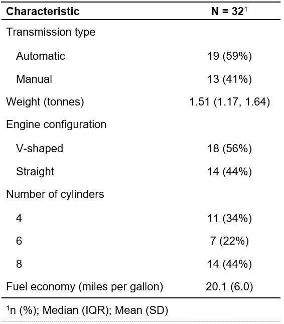
The code below uses the cars dataset we created and produces a table of descriptive statistics below for all the variables in this dataset. The table is produced in a Microsoft Word document called Descriptives Table 1. However, the path to this file will need to be changed to a location on your computer.

#Base this table on the 'cars' dataset
#Specify which variables are continuous and categorical
#Specify the name to use in the table for each variable
#State the descriptive statistics to use for each variable
#Specify the file path and file name for the Word document
tbl_summary(cars, 
  type = list(c(wt, mpg) ~ "continuous", c(am, vs, cyl) ~ "categorical"),
  label = list(
       am ~ "Transmission type",
       wt ~ "Weight (tonnes)",
       vs ~ "Engine configuration",
       cyl ~ "Number of cylinders",
       mpg ~ "Fuel economy (miles per gallon)"),
  statistic = list(
      c(mpg) ~ "{mean} ({sd})",
      c(wt) ~ "{median} ({p25}, {p75})",
      c(am, vs, cyl) ~ "{n} ({p}%)")
) %>%
as_flex_table() %>%
flextable::save_as_docx(path="C:/Users/ldw1c13/Documents/Descriptives Table 1.docx")

> Download this table in a Word document file.

To produce the table as a HTML file instead of a Word document, the packages flextable and officer do not need to be installed or loaded and the code in red above can be omitted.

 

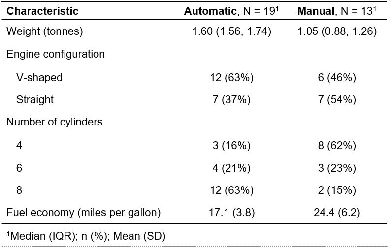
The code below uses the same dataset but produces a descriptive statistics table which is stratified according to transmission type (automatic or manual). In scientific studies, descriptive statistics are often shown separately for two groups if the aim is to compare these statistics between the two groups. For example, it may be of interest to compare participant characteristics between the control arm and intervention arm of a clinical trial. Another reason to stratify would be if certain characteristics are likely to differ greatly between the two groups; examples include descriptive statistics for weight and height between men and women.

#Stratify the above table according to transmission type
#Specify the stratification variable using ‘by = am’ 
tbl_summary(cars, 
  by = am,
  type = list(c(wt, mpg) ~ "continuous", c(vs, cyl) ~ "categorical"),
  label = list(
       wt ~ "Weight (tonnes)",
       vs ~ "Engine configuration",
       cyl ~ "Number of cylinders",
       mpg ~ "Fuel economy (miles per gallon)"),
  statistic = list(
      c(mpg) ~ "{mean} ({sd})",
      c(wt) ~ "{median} ({p25}, {p75})",
      c(vs, cyl) ~ "{n} ({p}%)")
) %>%
as_flex_table() %>%
flextable::save_as_docx(path="C:/Users/ldw1c13/Documents/Descriptives Table 2.docx")

> Download this table in a Word document file.

 

Produce tables of output from a linear regression model

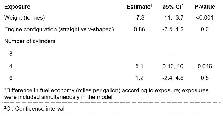
The code below creates a table containing the estimates, 95% confidence intervals and p-values from a multivariable linear regression model. The outcome variable is fuel economy in miles per gallon; exposures are weight, engine configuration and number of cylinders. To aid interpretation, we have changed the reference category for number of cylinders to the ‘8 cylinder’ category.

#Define the model ‘m1’ and use it in the regression table
#Specify the name to use in the table for each exposure
#Do not display the intercept in the table
#Only show one row for the binary exposure engine configuration
#Modify column headings and footnotes
m1 <- lm(mpg ~ wt + vs + relevel(cyl, ref = "8"), data=cars)
tbl_regression(m1,
    label = list(
       wt ~ "Weight (tonnes)",
       vs ~ "Engine configuration (straight vs v-shaped)",
       'relevel(cyl, ref = "8")' ~ "Number of cylinders"),
       intercept = FALSE,
       show_single_row = c(vs)
) %>% 
modify_header(label = "**Exposure**", estimate = "**Estimate**", ci = "**95% CI**", p.value = "**P-value**") %>%
modify_footnote(ci = "CI: Confidence interval", abbreviation = TRUE) %>%
modify_footnote(estimate ~ "Difference in fuel economy (miles per gallon) according to exposure; exposures were included simultaneously in the model") %>%
as_flex_table() %>%
flextable::save_as_docx(path="C:/Users/ldw1c13/Documents/Regression Table 1.docx")

> Download this table in a Word document file.

The table above shows that each extra tonne in weight was associated with a reduction in fuel economy of 7.3 (95% CI: 3.7, 11) miles per gallon after adjustment for engine configuration and number of cylinders.

Produce tables of output from a logistic regression model

The code below creates a table containing the odds ratios, 95% confidence intervals and p-values from a multivariable logistic regression model. The outcome variable is the binary variable transmission (automatic or manual); exposures are fuel economy in miles per gallon and engine configuration.

#Define the logistic regression model ‘m2’ and use it in the regression table
#Display exponentiated coefficients (odds ratios) in the table
m2 <- glm(am ~ mpg + vs, data=cars, family=binomial)
tbl_regression(m2, exponentiate=TRUE,
    label = list(
       mpg ~ "Fuel economy (miles per gallon)",
       vs ~ "Engine configuration (straight vs v-shaped)"),
       intercept = FALSE,
       show_single_row = c(vs)
) %>% 
modify_header(label = "**Exposure**", estimate = "**OR**", ci = "**95% CI**", p.value = "**P-value**") %>%
modify_footnote(estimate = "OR: Odds ratio", abbreviation = TRUE) %>%
modify_footnote(ci = "CI: Confidence interval", abbreviation = TRUE) %>%
modify_footnote(estimate ~ "Odds ratios for manual transmission according to exposures; exposures were included simultaneously in the model") %>%
as_flex_table() %>%
flextable::save_as_docx(path="C:/Users/ldw1c13/Documents/Regression Table 2.docx")

> Download this table in a Word document file.

This table shows that each mile per gallon increase in fuel economy was associated with an increase in the odds of a vehicle having manual transmission by a factor of 1.71 (95%CI: 1.26, 2.78) after adjusting for engine configuration.

 

One of the authors of the package gtsummary has provided detailed information about this package on the following website: https://www.danieldsjoberg.com/gtsummary/. This website includes additional information on how to further modify the output of descriptive statistics and regression tables in R which have been created using this package.

About the author

Dr Leo Westbury is a Statistician / Senior Research Fellow at the MRC Lifecourse Epidemiology Centre (University of Southampton). His research focuses on the lifecourse epidemiology of musculoskeletal ageing. This involves implementing statistical methods to explore determinants and examine health-related consequences of poor or declining musculoskeletal health in older age.

Primary author profile page

• Published on: 1 February 2024
• Event hosted by: Southampton
• Keywords: Automated Outputs | R Programming | Statistical Tables | gtsummary Package | Data Analysis | R |
• To cite this resource:

  Leo Westbury. (2024). Producing Automated Outputs (using R). National Centre for Research Methods online learning resource. Available at https://www.ncrm.ac.uk/resources/online/all/?id=20832 [accessed: 22 November 2024]

⌃
BACK TO TOP